XFLR5

WING ANALASYS

Before simulating a 3D wing, I first had to analyze the 2D cross-section (the airfoil) to generate the "performance lookup tables" (Polars) that the 3D solver requires.
I used a custom airfoil and I set up a Batch Analysis (Image 11) to simulate this airfoil across a range of Reynolds Numbers.

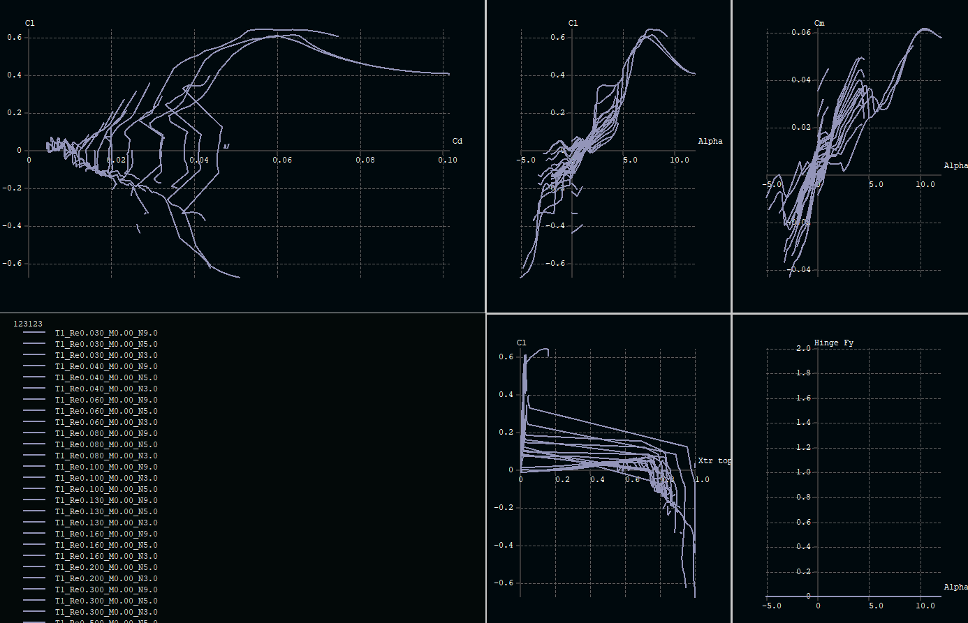
The resulting graphs show the Cl vs Cd and Cl vs α.

The curves are quite jagged and this indicates that at these low Reynolds numbers, the airflow over this specific airfoil is experiencing numerical instability in the XFoil solver. This introduces some noise into the final 3D data but provides the necessary baseline for viscous drag calculations.

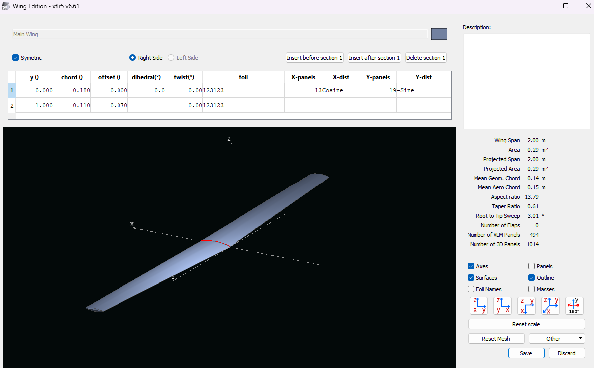
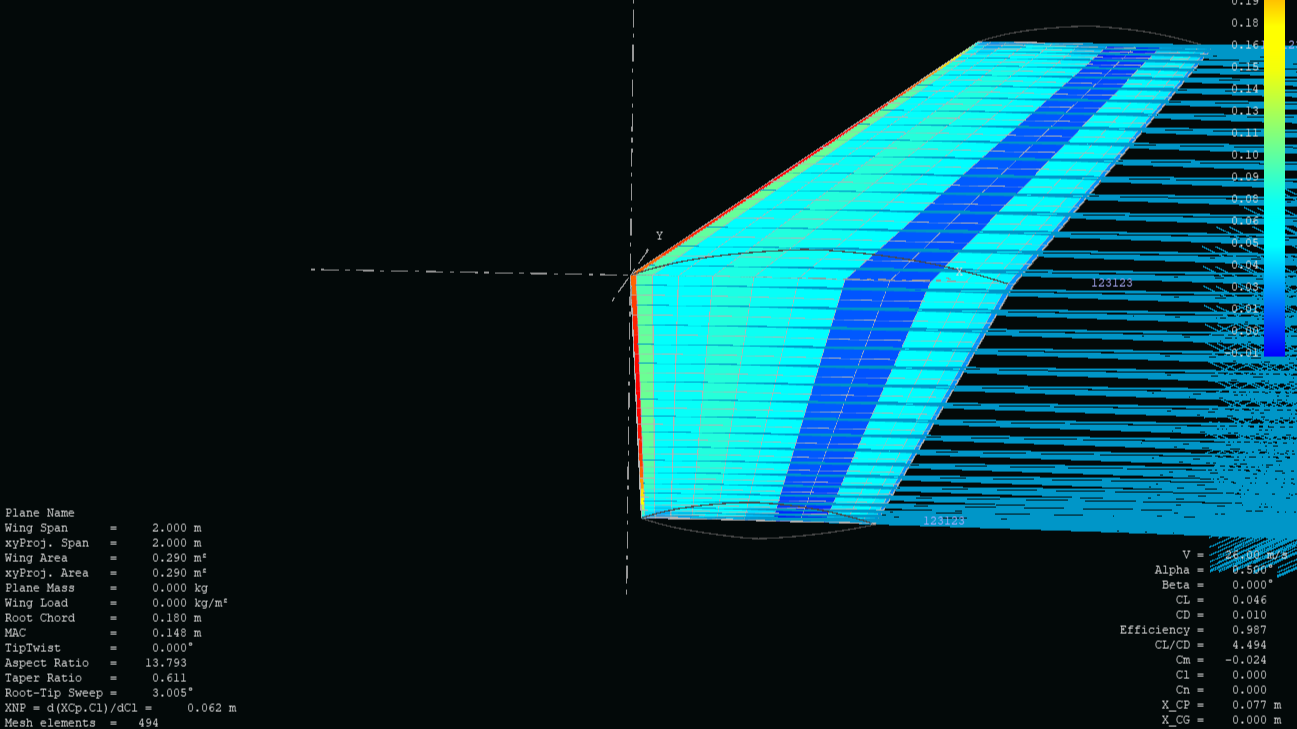
Next, I defined the physical shape of the wing in the "Wing Edition" tab. I created a wing with a 2.00 meter span. This resulted in a High Aspect Ratio wing (AR=13.79), which is typical for high-efficiency UAVs. The Taper Ratio is 0.610.61, which is a good compromise between structural weight and aerodynamic efficiency.

With the geometry and 2D polars ready, I moved to the 3D analysis environment to simulate flight. I selected Type 1 (Fixed Speed) at 26 m/s. This simulates the drone cruising at a specific velocity while the Angle of Attack changes. I used VLM1 (Vortex Lattice Method). This method is excellent for calculating Lift and Induced Drag. I enabled "Viscous" options to include the skin friction drag calculated in Phase 1. I ran a sequence of angles of attack from −7∘to+6∘to see how the plane performs during a dive, level flight, and climb.

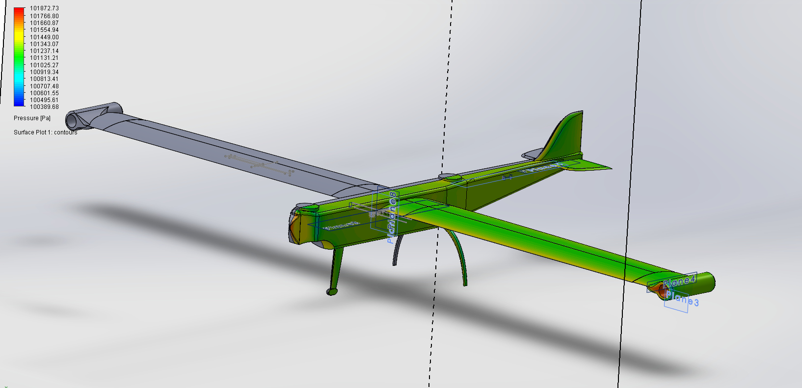
The wing surface is coloured by pressure. Red/Orange represents high pressure , and Blue/Cyan represents low pressure. The gradient is smooth across the span. You can see the high pressure on the bottom surface and suction on the top. This pressure difference is physically what generates the lift. The intensity fades toward the tips, which is expected as pressure equalizes at the wingtips creating vortices.

The Local Lift graph (bottom middle) forms a nice arch. This shape is close to an Elliptical Lift Distribution, which is the theoretical ideal for minimizing Induced Drag. The Cl graph (top right) is relatively flat, meaning the wing is working equally hard across the whole span, preventing one section from stalling way before another.

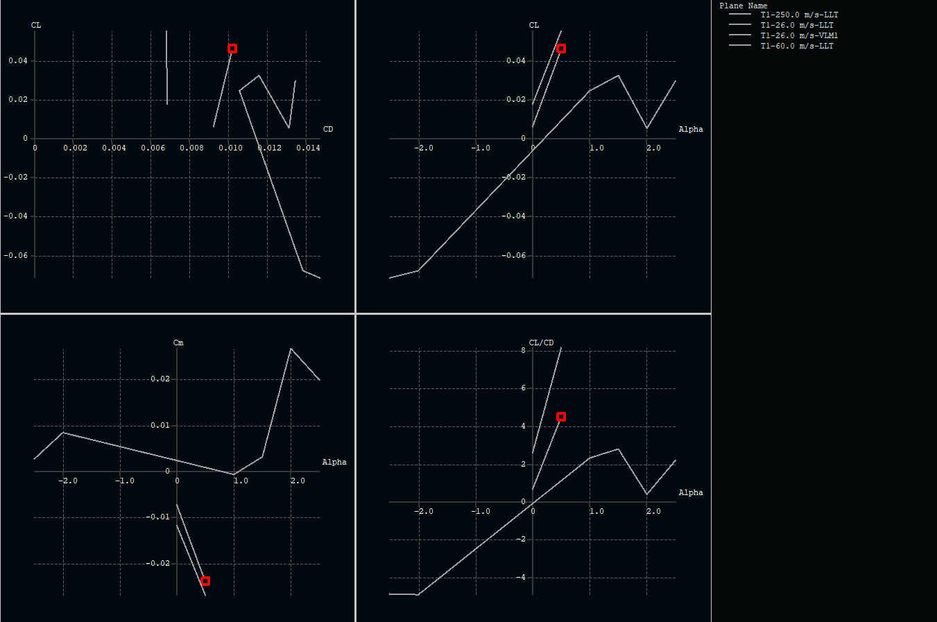
The Cl vs Cd polar displays a distinct 'drag bucket,' though it exhibits characteristic jaggedness due to low Reynolds number effects and the formation of laminar separation bubbles. The lift curve (Cl vs a) maintains a consistent linear slope, confirming stable flow within the primary flight envelope. Peak aerodynamic efficiency (L/D) is sharply defined at a low angle of attack (a ≈ 0.5° to 1.0°), validating the Ocelex wing's optimization for high-speed cruise efficiency rather than low-speed loitering.

Regarding longitudinal trim, the Cm vs. a graph shows a baseline pitching moment of approximately -0.01 at 0°. This nose-down torque is expected for a cambered high-aspect-ratio wing and confirms the requirement for a horizontal stabilizer to achieve equilibrium. Notably, the instability spike observed between 1° and 2° correlates with the laminar separation artifacts seen in 2D polars; this transition region necessitates a robust tail design to maintain longitudinal authority and suppress non-linear pitching tendencies during cruise.

FRAME CREATION & PRESSURE SIMULATION

PROPELLER ANALYSIS

THROTTLE TILT